鐵人賽2019 Day07 進階幾何資料處理

今天的主題是延續Day04 幾何資料基本運算，記錄一下在GIS向量資料中，可能會碰到但比較進階的幾何處理，今天的測試主要是圍繞在shapely的應用，shapely在Geopandas也有依賴，因此相關操作可以互相延伸。

在線資料中內插點

shapely的interpolate滿方便的，我們知道向量資料包含了點線面，線與面是由一序列的點組成的，shapely的interpolate提供了一個方法，可以在這樣的序列資料中，沿著序列的方向內插一個點。

有關向量資料，請參考[Day 11] WebGIS中的向量圖層-除了點資料以外的幾何

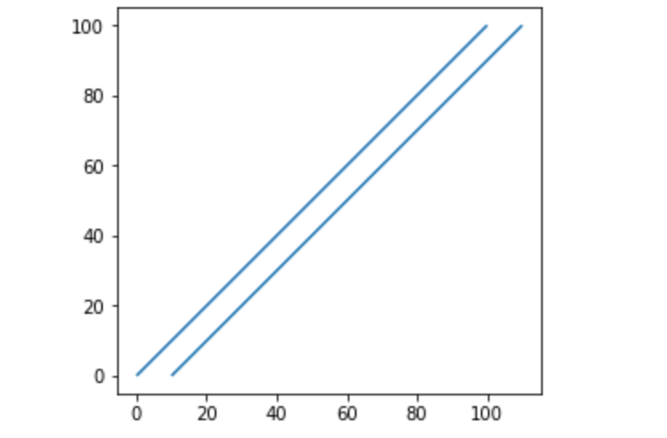
為此，我們先產生兩個線做說明

import geopandas as gpd
from shapely.geometry import LineString,Point
line1 = LineString([(0, 0), (50, 50), (100, 100)]) 
line2 = LineString([(10, 0), (60, 50), (110, 100)]) 
lines = gpd.GeoDataFrame()
lines['geometry'] = [line1,line2]
lines.plot()

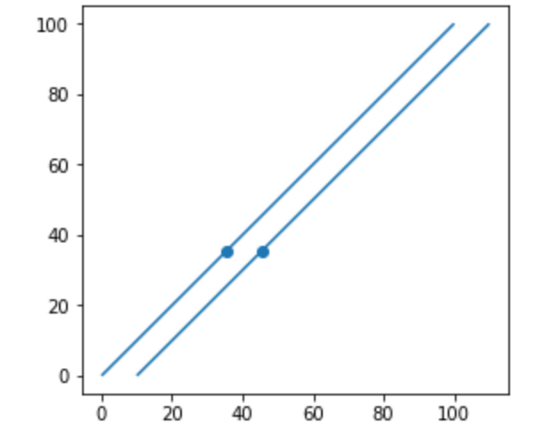
接著分別對資料做內插，其中distance是要內插的距離

base=lines.plot()
points = gpd.GeoDataFrame()
points['geometry'] = [row['geometry'].interpolate(50) for idx,row in df.iterrows()]
points.plot(ax=base)

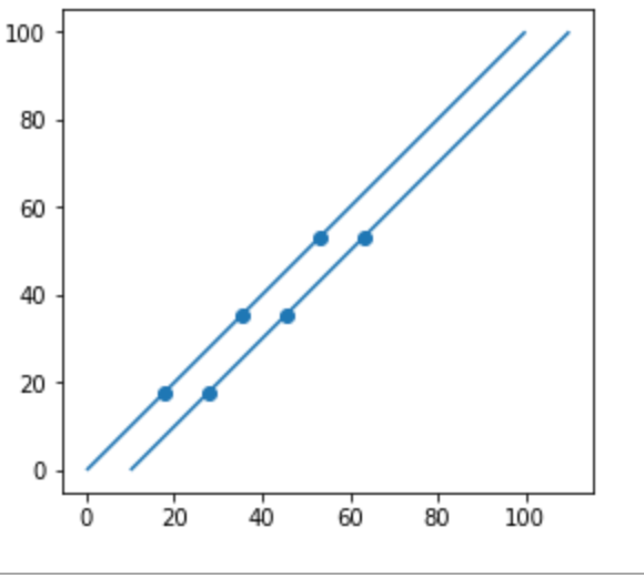
內插多個點

base=lines.plot()
points = gpd.GeoDataFrame()
intpoints=[row['geometry'].interpolate(50) for idx,row in df.iterrows()]
intpoints+=[row['geometry'].interpolate(25) for idx,row in df.iterrows()]
intpoints+=[row['geometry'].interpolate(75) for idx,row in df.iterrows()]
points['geometry'] = intpoints
points.plot(ax=base)

project

shapely的project這個方法會回傳線資料對與一個點的投影距離，
直接用案例來看:

LineString([(0, 0), (50, 50), (100, 100)]).project(Point(50,0))

回傳值=35.3553390

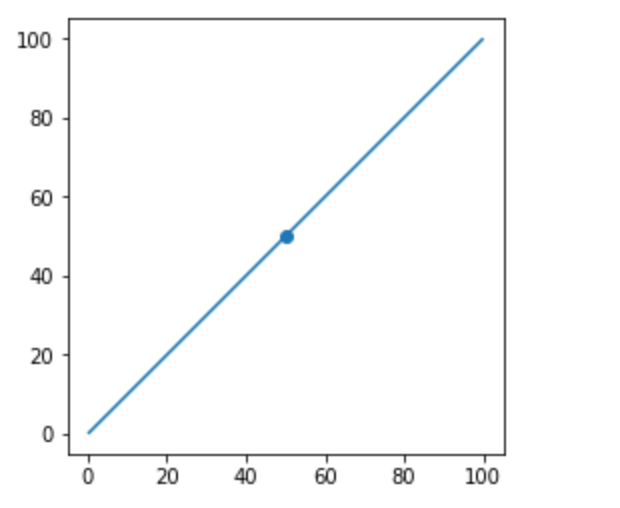
我們把圖畫出來

lines = gpd.GeoDataFrame()
lines['geometry'] = [LineString([(0, 0), (50, 50), (100, 100)])]
base=lines.plot()

points = gpd.GeoDataFrame()
points['geometry'] = [Point(50,0)]
points.plot(ax=base)

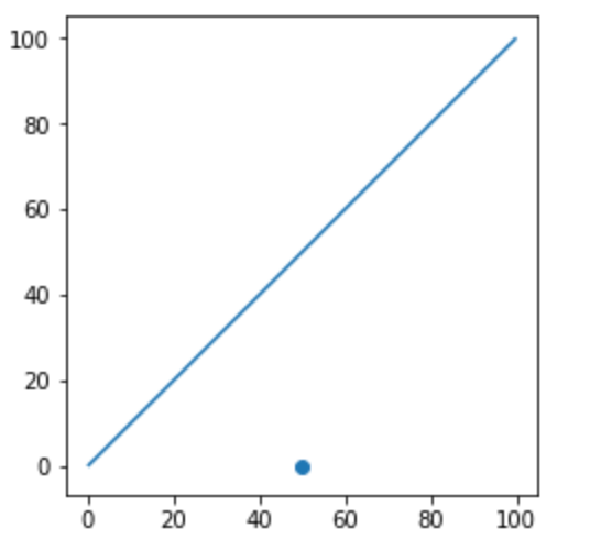
project方法提供的，是(50,0)這個點，投影在線上的點p，這個點p距離線的原點(0,0)的距離

再看一個例子，這次我們特意把點指定在線上(投影就是自己)

lines = gpd.GeoDataFrame()
lines['geometry'] = [LineString([(0, 0), (50, 50), (100, 100)])]
base=lines.plot()

points = gpd.GeoDataFrame()
points['geometry'] = [Point(50,50)]
points.plot(ax=base)
LineString([(0, 0), (50, 50), (100, 100)]).project(Point(50,50))

回傳值=70.710678

其中，70.710678其實就是(50,50)到這條線的原點(0,0)的距離

de-9im-relationships

de-9im全名是(Dimensionally Extended nine-Intersection Model)，是一個GIS位向關係描述的模型及標轉，這個模型描述了兩個幾何物件的關係，它把兩個幾何物件的關係以物件的I(Interior),B(Boundary),E(Exterior)，兩物件之間的幾何關係以此3*3內的關係來判斷，這個矩陣就是de-9im，以下圖為例：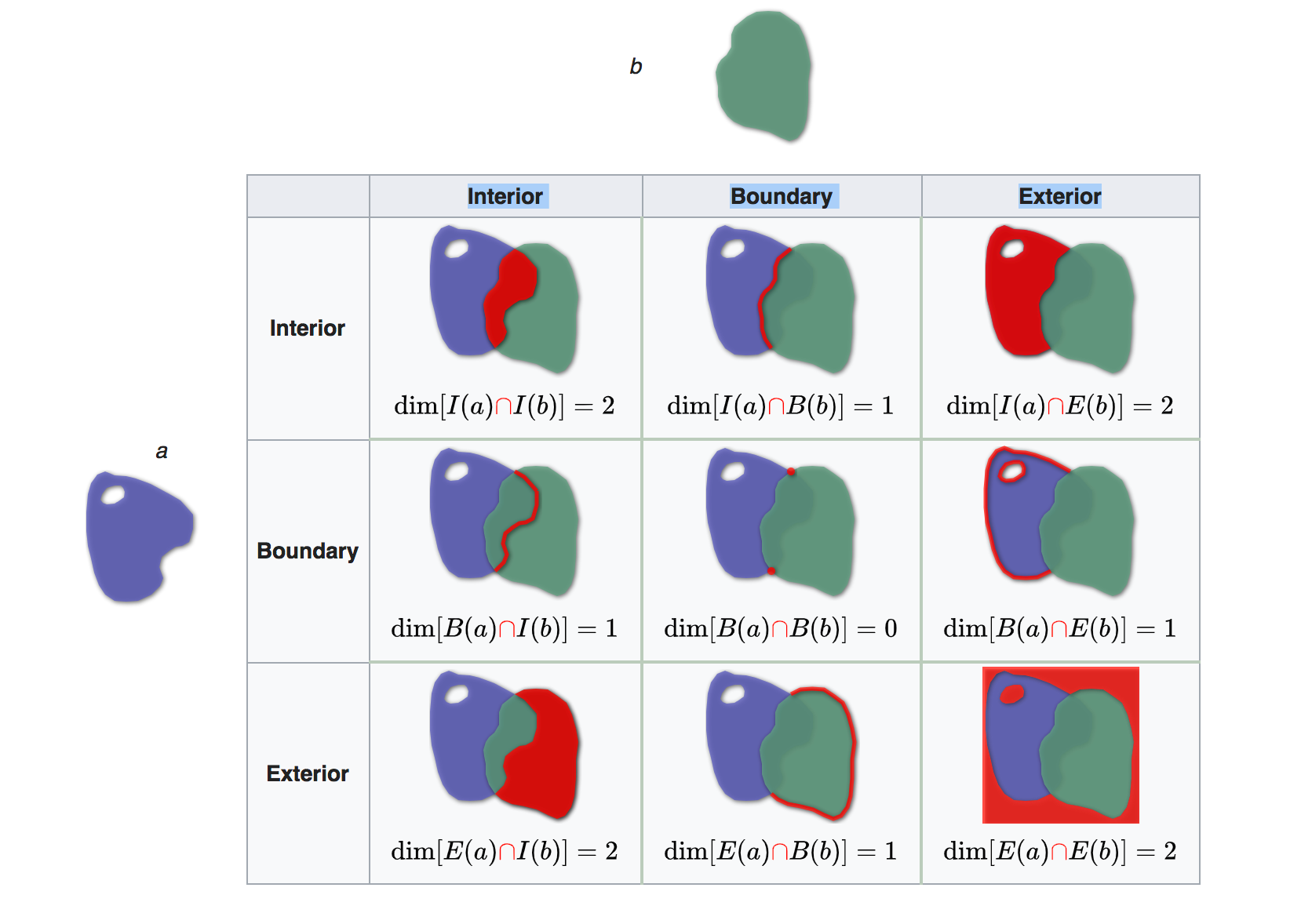

[取自DE-9IM - Wikipedia]

上圖範例中，a及b為兩個面，他們之間的關係按I, B, E三個觀點切入，在矩陣內的Dim()函數表示此關係的維度。如果相交部分點則為0，線則為一維，dim()=1，面則dim()=2，而不相交為dim()=-1，de-9im的讀法可以中從上往下、從左往右將數字集合起來如本案例的212101212，這串數字就用來表達這兩個物件的關係。

這樣的模型再把它簡化一點，我們把維度dim()簡化成相交(0,1,2維)與不相交(-1)，分別以T與F表示，配合I, B, E三個角度的判斷，這樣也可以拿來描述兩個幾何物件的關係。

另外，我們常用的幾何物件關係的描述，若以de-9im表示，
其實並不需要9個元素都判斷就可以判斷他們是否符合這個關係，
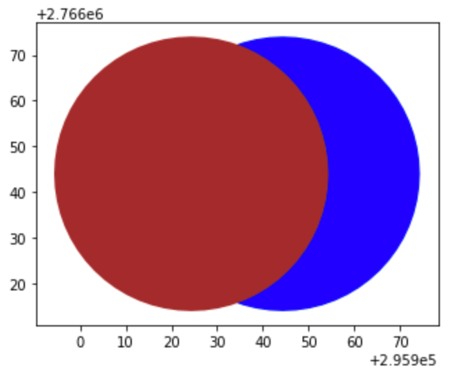
例如以上兩個面相交的例子：
實際上它是
TTTTTTTTT
事實上只要知道第一個T，就可以決定這種關係
T********

又例如兩個面分離(Disjoint)，他應符合：
FF*FF****
我們直接來測試，把第三天的資料再來拿看看
更多的幾何關係可以參考Spatial Relations Defined

p1=gpd.read_file('output/Library.shp',encoding='utf-8').head(1)
p1.crs = {'init' :'epsg:4326'} # 避免資料沒設，這邊再重新給一次
p1=p1.to_crs(epsg=3826)
p1['geometry']=p1.buffer(30).translate(xoff=20.0, yoff=0.0)

p2=gpd.read_file('output/Library.shp',encoding='utf-8').head(1)
p2.crs = {'init' :'epsg:4326'} # 避免資料沒設，這邊再重新給一次
p2=p2.to_crs(epsg=3826)
p2['geometry']=p2.buffer(30)
base=p1.plot(color='blue')
p2.plot(ax=base,color='brown')

由於Geopandas的geometry是依賴於shapely，使用relate這個方法
看看他的de-9im的值

p1.at[0,'geometry'].relate(p2.at[0,'geometry'])

回傳值=212101212

今天的相關測試可以參考GitHub